Determining an orbit from one radar observation was the chapter in Fundamentals of Astrodynamics by Bates, that I flipped to when I took the book off of my grandpa’s shelf. I flipped through the introduction to the section, and was fascinated about the Doppler effect. Being experienced only in High School introductory physics at the time, I only knew about the Doppler shift in the context of red/blue and the sound a F1 car made as it zoomed past. Seeing that we could determine an orbit of a satelite all the way out in space with just these basic data points fascinated me, and I sat down and worked my way through the rest of the book. It’s been about 3 years since then and I finally felt like I had the calculus and linear algebra skills to implement the projects in the back of the book. So over a weekend, I hacked on the code and algorithms to turn a radar observation into an orbit.

I plan to make this the first in a series of 5 posts:

• Determination from a radar observation

• Determination from position vectors

• Determination from optical sightings

  • Possibly turn this into a project post with a raspberry pi, and a DSLR, determining the orbit of satelites that pass overhead.

• Finally, how to improve the accuracy of these preliminary orbits.

The problem

With an introduction out of the way, let’s now focus on the problem at hand. There are a series of radar observation sites around the world, they can be found in a variety of locations; scientific observatories, military bases, airports, and more.

enough with the boring intro that everyone skips, on to the code!

The first step was processing and entering the data, for that I decided that a CSV was the best choice in order to process multiple data points, easier data input, and also use Pandas which handles CSV’s with remarkable ease. For this project, Python’s built in reader will do the job just fine. The code is long, and not very substantive, but it is in the Github repository if you are curious.

Data comes in many different types, and as a reciever of data it is my priority to make sure that all data is in a usable format, and specifically for this project, the proper units.

So after multiplication and division by conversion factors, if statements, and string trimming, I arrive at perfectly clean usable data.

The math!

Let’s define some constants first to use in our calculations

# setting up an inertial reference frame
wE = .00089 # rad/second
omega = [0,0,wE] # earth rotates on the Z axis

# measurement of the earths axial tilt in 1970, important for ascending node calculations
J1970 = time.Time('J1970', scale='utc')

# To compute earths oblateness factor
eccentricity = 0.08182
equatorial_radius = 6378.145 # km
polar_radius = 6356.785 # km

Let’s go through these one by one and explain.

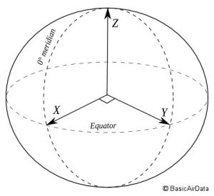
• wE describes the angular rotation that a point on the earth travels. The array omega represents the rotating coordinates of the earth. In a right hand coordinate system, the z coordinate that rotates. As shown in the image below.

Next we have the time epoch. As the earth precesses on it’s axis, the measurements for celestial coordinate systems change. Namely; right ascension, and the vernal equinox direction. Defining a standar for the axial ‘tilt’ of the earth is necessary for precise measurements and scientific reproducibility.

Finally, we have a couple measurements of the earth’s elliptical properties. As the earth rotates around it’s Z axis, there exists a certain oblateness. Just as your arms naturally want to spread out as you spin, the angular momentum at the equator is sufficient to pull the earth outwards also. We can approximate this ‘stretch’ with an ellipse fairly accurately. Taking the equatorial radius, the distance around the equator, and then the polar radius, the distance around the poles, we arrive at an eccentricity value using basic ellipse formulas.

Next, let’s get down and dirty and determine a topocentric state vector, pointing from the radar station to the tracked object, and velocity from the object, pointing in the direction of travel. Taking all of the radar data, we can determine these vectors fairly simply with the trigonometry of this diagram.

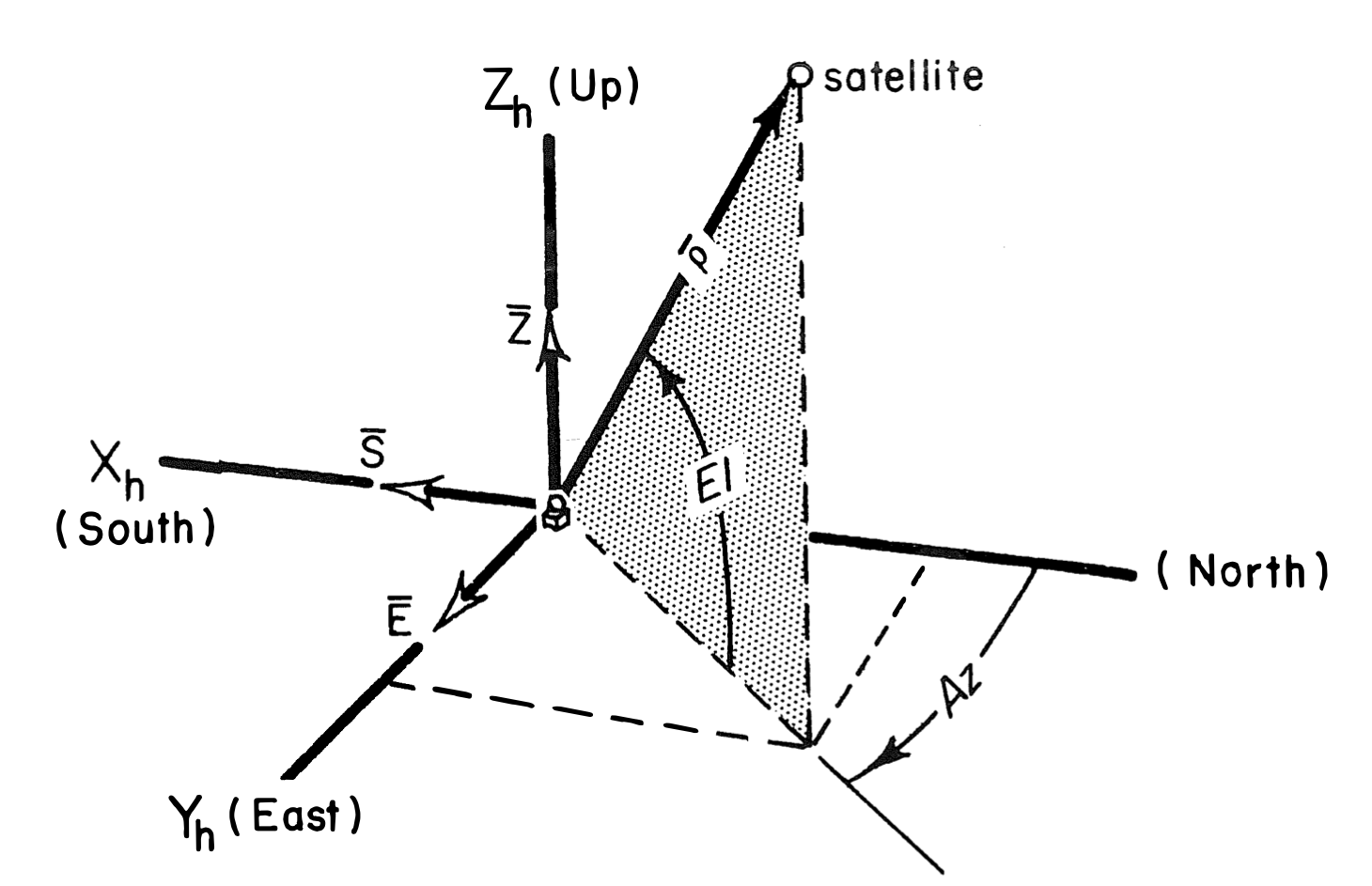
The position vector of the satellite relative to the radar site:

and the velocity is given by it’s derivative:

The code:

def compute_position_and_velocity_vectors_topocentric(range, range_rate, elevation, elevation_rate, azimuth, azimuth_rate):    

    rho_S = -1 * range * math.cos(elevation) * math.cos(azimuth)
    rho_E = range * math.cos(elevation) * math.sin(azimuth)
    rho_Z = range * math.sin(elevation)

    rho = np.array([rho_S, rho_E, rho_Z])

    rho_dot_S = -1 * range_rate * math.cos(elevation) * math.cos(azimuth) + range * math.sin(elevation) * elevation_rate * math.cos(azimuth) + range * math.cos(elevation) * math.sin(azimuth) * azimuth_rate
    rho_dot_E = range_rate * math.cos(elevation) * math.sin(azimuth) - range * math.sin(elevation) * elevation_rate * math.sin(azimuth) + range * math.cos(elevation) * math.cos(azimuth) * azimuth_rate
    rho_dot_Z = range_rate * math.sin(elevation) + range * math.cos(elevation) * elevation_rate
    
    rho_dot = np.array([rho_dot_S, rho_dot_E, rho_dot_Z])

    return rho, rho_dot

Now to truly make this a global state vector of the satelite, we must transform from topocentric, earth’s surface, coordinates to geocentric, earth-centered, coordinates. Now if the earth was perfectly spherical that would be as simple as adding an earth radius \(R\) to \(\rho_{Z}\), the zenith of the observing site, as can be determined visually from the below image.

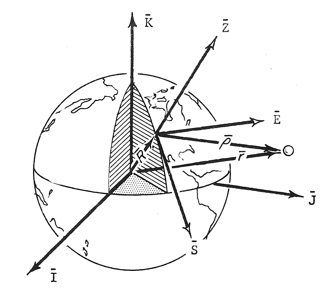
Unfortunately, it isn’t quite that simple. We defined in the first section a couple variables that tell us about the eccentricity of the earth, we will use that now to compute the radius of the earth at any location, using geodetic latitude. Coordinates on the ellipse can be described using latitude, \(L\), the eccentricity, \(e\), an angle \(\theta\) describing the local sidereal time, more specifically the angle between the observer and the vernal equinox, a height, \(H\) above sea level, and the equatorial radius of the earth, \(a_{e}\).

def compute_station_coords_ellipsoid(lst_time, lat, elevation_sea_level):

    x = abs(1 / ( math.sqrt(1 - math.pow(eccentricity,2) * math.sin(lat))) + elevation_sea_level) * math.cos(lat)
    z = abs(1 / ( math.sqrt(1 - math.pow(eccentricity,2) * math.sin(lat))) + elevation_sea_level) * math.sin(lat)
    R = array([ x * math.cos(lst_time), x * math.sin(lst_time), z])
    return R

Now that we have our station coordinates, let’s set up our transformation matrix so that we can rotate from SEZ to IJK coordinate systems. The SEZ coordinate system is what we originally defined for our topocentric vectors. Now let’s dig underground and define a much more universal (or global, since whilst talking about space one can never be too specific ;) ) transformation to the center of the earth.

Euler angles, presented in the transformation matrix below, defined as \(D\), can be calculated based on rotating one vector at a time until the proper orientation is reached. [2] Using the geometry of our above figures, we use our geodetic latitude, and local sidereal time at the site to rotate our coordinates to a geocentric perspective.

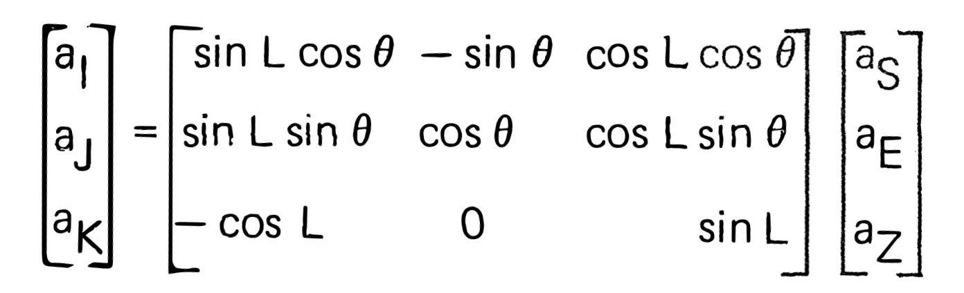
From this matrix, we can easily define the operations necessary to rotate our coordinate reference frame. Dotting \(r\) and \(D\), and \(v\) and \(D\).

With just one more step we arrive at our solution, since the earth is rotating relative to the satellite as well, we must factor this into the velocity. This is given simply by the following:

def compute_r_v_geocentric(r_topo, v_topo, lat, lst_time, elevation_sea_level):
    # Here we compute the site coordinates(using the above function), and add them to the topocentric position vector.
    R = compute_station_coords_ellipsoid(lst_time, lat, elevation_sea_level) 
    r_topo += R
    
    # define transformation matrix
    rotation_matrix = array([
        [math.sin(lat) * math.cos(lst_time), -1 * math.sin(lst_time), math.cos(lat) * math.cos(lst_time)],
        [math.sin(lat) * math.sin(lst_time), math.cos(lst_time), math.cos(lat) * math.sin(lst_time)],
        [-1 * math.cos(lat), 0, math.sin(lat)]
    ])

    # convert (3,) array to (1,3) to dot with rotation_matrix
    rho_3_vector = np.array(r_topo)
    rho_dot_3_vector = np.array(v_topo)

    r = dot(rotation_matrix, rho_3_vector)
    rho_dot = dot(rotation_matrix, rho_dot_3_vector)

    v = rho_dot + cross(omega_wE, r)

References

• Fundamentals of Astrodynamics (text)
• European Space Academy (ESA) Space Debris Radar
• space observation radar TIRA (Tracking and Imaging Radar)
• Axial Precession Youtube
• Euler Angle summary Youtube