Introduction

I was introduced to an app on my phone that uses all of the sensors to record interesting physics data. On the train to work the other day I opened up the app to record data from the 3 axes of accelerometers. I’ve been studying integrals and the intuition that a summed acceleration curve equals the velocity finally hit me.

It’s so simple but in my first calculus class, we studied that the derivative of velocity is acceleration. Okay, but that just didn’t make much intuitive sense to me at the time, other than the basic definition that the rate of change of velocity would equal acceleration I had no concept for what that felt or looked like. One of my good friends alwyas said that once you can hold something in your minds eye, turn it around, examine every inch of it, only then can you fully begin to understand something.

The idea was just as they teach it in class; that for every infinitesimal moment of acceleration, there in turn is some resulting change in velocity. Take for example a quick exponential acceleration graph. What would the velocity be after 5 seconds? For the logistic function \(\frac { L }{ 1+e^{-k(x-x_0)} }\)

Below is some code to graph the logistic function for our basic acceleration values. First it grows, exponentially, and then as it nears a maximum value, slows the growth rate.

import matplotlib.pyplot as plt
import numpy as np

x = []
y = []
duration = 200
accuracy = 20
e_incrementer = duration/accuracy # break down into small timesteps

step_size = e_incrementer

for i in range(duration):
    x.append(i)
    y.append((duration/10)/(1 + np.e ** (-.05 * (i - duration/2)))) # a logistic curve. modelling slowing acceleration as max speed is reached.
    
plt.plot(x,y)
plt.show()
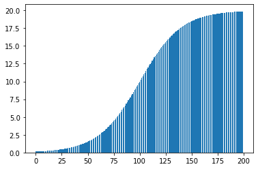
plt.bar(x,y)

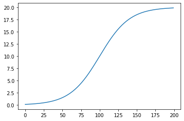
The first graph is our acceleration curve, and the second is an approximate integral of this curve. Since the area underneath a curve is traditionally found by taking infinitesimal rectangles, I modeled this with bars that fits our curve. Now to find the velocity, we simply take the width of each rectangle and multiply it by the height of the function at that point. *note that there are many different ways to numerically calculate integrals using quadrature that I plan to cover in the future, but for now this satisfies our requirements for a basic intuition

area = 0
for i in range(accuracy):

    # using the rectangle rule, we evaluate the function at each small step, multiply, and add to a running total
    e_to_t = (duration/10)/(1 + np.e ** (-.05 * (e_incrementer - duration/2)))
        
    area += step_size * (e_to_t)
    
    e_incrementer += e_incrementer


print(area)

import pandas as pd
import matplotlib.pyplot as plt
import numpy as np

data = pd.read_csv('data/accel_data.csv')
y_accel = data['y']
x_accel = data['x']
z_accel = data['z']
time_series_y = pd.Series(y_accel)
time_series_x = pd.Series(x_accel)
time_series_z = pd.Series(z_accel)
# the results are off by .1 ish... The data looks a lot better like this
time_series_y = time_series_y.subtract(.1, axis=0)

velocity = time_series_y.cumsum()
velocity.plot()

y_accel = y_accel.subtract(.1, axis=0)
y_accel = y_accel.multiply(1000, axis=0)
y_accel.plot()